Assignment Five: Correlation
Goals of Assignment Five
Create a Scatterplot with Trendline in Excel
Calculate Correlations Using SPSS
Interpret Correlations from a Scatterplot and SPSS Output
Use the US Census Site to Download Data and Shapefiles
Join US Census Data and Other Data
Report Results


Part I: Correlation

Introduction

A scatterplot was created using data, consisting of sound levels in decibels and distance of feet, provided by Dr. Ryan Weichelt and a trendline added using Microsoft Excel (Figure 2). A correlation analysis was then run in SPSS, with the results presented in Figure 3.

Definitions 
Scatterplot: Diagram representing value displays for two variables using Cartesian coordinate plots, with one variable acting as the X value and one acting as the Y value. The trendline represents the direction of the relationship with a downward-trending slope meaning a negative relationship and an upward-trending slope meaning a positive.

Correlation: Numerical representation between pairs of variables. Correlations test the strength of the relationship between the variables, with a value of +1 representing a perfect positive relationship (as X increases Y also increases) and a value of -1 representing a perfect negative relationship (as X increases Y decreases, for example). A correlation only shows the relationship between two variables at a time but a correlation matrix (Figure 3) allows for several correlations to be presented in one output file.

Strength of Correlations:

Figure 1: Correlation Strengths
https://blog.majestic.com/case-studies/majesticseo-beginners-guide-to-correlation-part-5/

a. Create a Scatterplot with trend line.

Figure 2: Scatterplot of Sound Level and Distance

b. Show the results of the Pearson Correlation using SPSS.

Figure 3: Pearson's r Correlation for Sound Level and Distance Variables

d. What is the hypothesis? 

Null Hypothesis: There is no linear relationship between sound level and distance.

Alternative Hypothesis: There is a linear relationship between sound level and distance.

e. Summarize your findings.

The scatterplot (Figure 2) shows a trendline that is decreasing as distance increases, suggesting a negative relationship between the two variables. This scatterplot is considered to represent a strong association as the data points are tightly packed along the trendline. The Pearson r Correlation (Figure 3) confirms this and the null hypothesis is rejected as our 2-tailed significance is .000, which is less than the significance level of .01. An r value of -.896 is considered a strong negative relationship; there is a decrease in sound levels at distance.  

Correlation Matrix

Figure 4: Correlation Matrix Between Ethnicity and Multiple Economic Variables, Detroit, USA

Hypothesis

For the sake of simplicity, one null hypothesis and one alternative hypothesis will be presented.

Null Hypothesis: There is no linear relationship between ethnicity (white, black, asian, hispanic) and bachelor's degrees, median household income, median home value, and job type (manufacturing, retail, and finance).
Alternative Hypothesis: There is a linear relationship between ethnicity (white, black, asian, hispanic) and bachelor's degrees, median household income, median home value, and job type (manufacturing, retail, and finance).

Results

All results use the data portrayed in Figure 4.

Ethnicity and Bachelor's Degree
The linear relationships between ethnicities, whites (r = .698), blacks (r = -.305), and Asians (r = .559), and bachelor's degree are all significant at the .01 level, two-tailed, while the linear relationship between Hispanics and bachelor's degree is not, with an r value of -.058. The null hypotheses would be rejected for all ethnic groups except for Hispanics, as the two-tailed significance is .068, which is greater than the significance level of .01. There is as significant linear relationship between whites, blacks, and Asians and bachelor's degrees but not between Hispanics and bachelor's degrees. Using Figure 1, the strength of each of these relationships can be assessed, so that an r of .698 is considered to represent a moderately strong positive relationship while an r of -.058 is considered to represent a very low strength negative relationship.

Ethnicity and Median Household Incomes
The linear relationships between ethnicities, whites (r = .554), blacks (r = -.408), and Asians (r = .388), and median household incomes are all significant at the .01 level, two-tailed, while the linear relationship between Hispanics (r = -.078) and median household income is significant at the .05 level, two-tailed. The null hypothesis was rejected for all ethnic groups as the two-tailed significance values are all less than the significance levels.

Ethnicity and Median Home Values
The linear relationship between ethnicities, whites (r = .486), blacks (r = -.362) Asians (r = .436). and Hispanics ( r = -.092), and median home values are all significant at the .01 level, two-tailed. The null hypothesis was rejected for all ethnic groups as there are significant linear relationships between all ethnicities and median home values.

Ethnicity and Manufacturing Jobs
Blacks (r = -.085) and Asians (r = .077) were the only ethnicities to have significant linear relationships at the .01 level of significance, two-tailed, and .05 level of significance, two-tailed, respectively. Both have very low correlation strengths. Whites (r = .011) and Hispanics (r = -.009) both have very low and insignificant correlation strengths. The null hypothesis was rejected for blacks and Asians but not for whites or Hispanics.

Ethnicity and Retail Jobs
Whites (r = .184), blacks (r = -.146), and Asians (r = .259) all have significant linear relationships at the .01 level of significance, two-tailed, while Hispanics (r = -.004), did not. The null hypothesis was rejected for whites, blacks, and Asians as there is a significant linear relationship between their ethnicities and retail jobs.

Ethnicity and Finance Jobs
Only Asians had a significant relationship with finance jobs (r = .097). Whites ( r = -.007), blacks (r = -.042), and Hispanics (r = -.034) all have very low negative correlations with finance jobs. The null would was rejected for Asians but not for the other three ethnic groups.

Conclusion

Whites and Asians have positive linear relationships between their ethnicities and what would be considered to be the preferred variables of bachelor's degrees, median household incomes, and median home values. Blacks and Hispanics have negative linear relationships with these preferred variables. It appears that whites and Asians are better educated, which may influence their higher positive correlations with median household income and median home values. Whites also have slightly stronger positive correlations with these three variables than Asians do. When it comes to jobs, blacks and Hispanics have negative relationships among the three job variables used in this analysis, while whites and Asians have positive linear relationships with these three job variables, except for finance, where whites have a very low negative linear relationship with that variable. We cannot imply causation from correlation but this data is very interesting. Blacks and Hispanics do not seem to attain the same level of education that whites and Asians do and also experience lower rates of employment in manufacturing, retail, and finance positions. It seems, stressing that ethnicity does not cause the linear relationships we see here, that there are reasons for these patterns that are observed here. It would take require a rigorous inferential analysis to determine what the potential causes of the discrepancies between ethnicity and these economic variables are.

Part II: Spatial Autocorrelation

Introduction

The Texas Election Commission (TEC) commissioner, Dr. Ryan Weichelt, wants to see if there is a clustering of voting patterns in the state of Texas by county. The results of this analysis, comparing the spatial patterns of percentage of democrat votes between the election of 1980 and 2012 and voter turnout in those elections, will be provided to the governor to see if election patterns have changed over the past 32 years. The TEC suggests that the determination of spatial autocorrelations will provide the data needed to see if a clustering is occurring. A spatial autocorrelation is a correlation of a variable with itself through space. For example, if there are counties nearer each other that are similar in levels of voter turnout in 1980, these counties would have a high, high relationship. The use of autocorrelation will determine if there are spatial patterns that exist between the variables that are to be examined for this analysis.

Figure 5: Moran's I Output

Dr. Ryan Weichelt

The output is placed into four quadrants of comparison. Each value, by counties this analysis, is compared to each other value and are placed in the following categories: 

High, High (+,+) areas that contain high values of a variable that are surrounded by areas that contain high values of a variable.

High, Low (+,-) areas that contain high values of a variable that are surrounded by areas that contain low values of a variable. Outliers

Low, High (-,+) areas that contain low values of a variable that are surrounded by areas that contain high values of a variable. Outliers.

Low, Low (-,-) areas that contain low values of a variable that are surrounded by areas that contain low values.

The value of Moran's I ranges from -1 to +1, like a Pearson's r correlation but, unlike a Pearson's r correlation, a negative or positive value does not imply the direction of the correlation but, rather, the degree to which a variable is clustered. A positive Moran's I is more clustered while a negative value is less clustered. Local indicators of spatial autocorrelation (LISA) maps provide a visual representation of clustering.  

Methodology

A Texas county shapefile and Hispanic population data by Texas county were downloaded as zip files from the United States Census Bureau at http://factfinder2.census.gov/faces/jsf/pages/index.xhtml. The percentage of Hispanic population by Texas county data from the population file was added to an Excel file provided by Dr. Ryan Weichelt that contained Texas election data for voter turnout and the percentage of the vote that for the Democratic candidate for the years 1980 and 2012. ArcMap was then opened and the Excel data file was joined to the Texas shapefile using Geo_ID. This data was exported as a new shapefile to be used in Geoda by clicking on "Data" then "Export Data" and "Save as Type" was changed to shapefile as Geoda can only open shapefiles. Geoda was then opened and "File" was clicked, followed by "New Project From" and the Texas shapefile was opened. Before a spatial autocorrelation could be performed, a spatial weight had to be created by going to "Tools" to "Weights Manager" and then to "Create". The "Add ID Variable" was then selected, which opens up "Add New ID Variable Name" followed by selecting "Add Variable". The final step was selecting "Rook Contiguity" under "Contiguity Weight" then clicking "Create". Using the "Cluster Map" box five Moran's I calculations were performed and the five output graphs and LISA maps were then added to the final report. SPSS was then used to perform a correlation matrix to better explain the data along with a map of Hispanic population percentages that was created from the mxd file created sy the beginning of this analysis, using a graduated colors scheme and the Jenks Natural Breaks (divided into 5 classes) classification method.     

Results

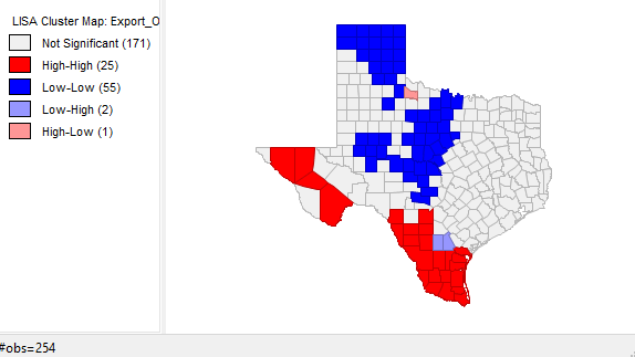
In 1980 (Figure 6), the Moran's I value is .468058 and high voter turnout is concentrated in the Texas panhandle and a few counties in central Texas while low voter turnout is clustered in the east and southern Texas along the Mexican border. There are four high-low counties and six low-high but the majority of counties in Texas show no significant clustering. In 2012 (Figure 7), the Moran's I value is even lower, at .335851, and there is an obvious decrease in the clustering of high-high counties but there is still a pronounced low-low clustering of voter turnout in southern Texas along the Mexican border and an additional clustering of low voter turnout in the western Texas panhandle that was not present during the presidential election of 1980. The majority of counties show no clustering. In 1980 (Figure 8), with a Moran's I value of .575173, the clustering of counties with high percentages of votes for the democrat candidate, occurs in the eastern and southern parts of Texas along the Mexican border. Areas of low percentages of votes for the democrat candidate are clustered in the western part of the Texas panhandle and in central Texas. There are very few counties that are high-low and low-high and the majority show no clustering. In 2012 (Figure 9), with a Moran's I value of .695853, sees a definite shift of clustering of higher democrat vote percentages from the east to the west along with a shift of low-low clustering from the western to northern panhandle along with an increase of clustering in central Texas of counties with low vote percentages in favor of democrats. There are only three counties that are high-low and low-high while the majority of counties show no clustering. The spatial analysis of Hispanic population by percentage (Figure 10) resulted in the highest Moran's I value of  .778655, which means that there is a significant clustering of Hispanic and non-Hispanic populations. The majority of the clustering of Hispanics is along the border with Mexico, in the western panhandle, and in one county surrounded by a majority non-Hispanic population. Majority non-Hispanic populations are clustered in the eastern part of the state and in one county in the western region of Texas. Figure 11 was produced to show the connections between low voter turnout and percentage democrat vote clusters in both 1980 and 2012; this chloropleth map shows the percentages of population that is Hispanic by Texas county. Voter turnout and voting pattern clusters match well with the counties along the Mexican border, which have higher percentages of Hispanic populations. The reverse holds true for areas with higher voter turnout and percentage of democrat vote. In 1980 voter turnout was clustered in northern and central Texas. In 2012 voter turnout was also clustered in these areas but to a lesser extent (note the lower Moran's I in 2102 voter turnout as compared to 1980 voter turnout). In 1980 and 2012 clusters of low percentages of democrat votes occurred mainly in the northern counties of Texas and counties of central Texas. These regions have lower percentages of Hispanic citizens. Figures 10 (clustering of populations) and 11 (chloropleth map of Hispanic populations by county percentages) when compared, match up very well. The western counties of Texas, especially along the border with Mexico, into the panhandle have higher percentages of Hispanic populations than the northern or eastern counties in Texas. It appears that Hispanics vote in lower numbers and, when they do vote, do so mainly for democrats. It also appears that voter turnout has decreased in counties that vote for democrats at higher percentages. To test these hypothesis a correlation matrix was created. This matrix is presented in Figure 12. The hypotheses were as follows:

Hypothesis Set 1

Null Hypothesis: There is no linear relationship between the percentage of Hispanics and four other variables: voter turnout in the presidential elections of 1980 or 2012, or percent democrat vote in the presidential elections of 1980 or 2012

Alternative Hypothesis: There is a linear relationship between the percentage of Hispanics and voter turnout 1980 or 2012 or percent democrat vote in 1980 or 2012.        

There is no linear relationship between percent democrat vote and percent Hispanic population (r = 

.093) for the presidential election of 1980, so the null was not rejected as the observed two-tail significance level of .139 is greater than the .01 level. There is however, a significant positive 

correlation between percent democrat vote and percent Hispanic population (r = .718), two-tailed, .01 significance level. There are also significant negative linear relationships between percent Hispanic 

populations and voter turnout in 1980 (r = -.407) and 2012 (r = -.718). It appears that while Hispanics have become more likely to vote for the democrat candidate, they are voting less in presidential elections. The null is rejected in both of these cases as the r correlations are both significant to the .01 level, two-tailed. 

Hypothesis Set 2

Null Hypothesis: There is no linear relationship between voter turnout by county (both 1980 and 2012) and percent democrat vote by county in the presidential elections of 1980 or 2012.

Alternative Hypothesis: There is a linear relationship between voter turnout by county (both 1980 and 2012) and percent democrat vote by county in the presidential elections of 1980 or 2012.

In 1980, the correlation between voter turnout and percent democrat is a negative linear relationship (r = -.612), significant to the .01 level, two-tailed, and the null was rejected. In 2012, the correlation between voter turnout and percent democrat is also a negative linear relationship (r = -.623), significant to the .01 level, two-tailed, and the null was rejected. This supports the observation that less people are voting in counties where democrats receive higher percentages of votes.   

Voter Turnout 1980

Figure 6: Moran's I and LISA Map of Voter Turnout in 1980

Voter Turnout 2012

Figure 7: Moran's I and LISA Map of Voter Turnout in 2012

Presidential Election, % Democrat Vote, 1980

Figure 8: Moran's I and LISA Map of Presidential Election 1980, Democrat Vote Percentage

Presidential Election, % Democrat Vote, 2012

Figure 9: Moran's I and LISA Map of Presidential Election 2012, Democrat Vote Percentage

% Hispanic

Figure 10: Moran's I and LISA Map, Hispanic Percentage of Population

Figure 11: Hispanic Population by Percentage, Texas, 2010 Census Data

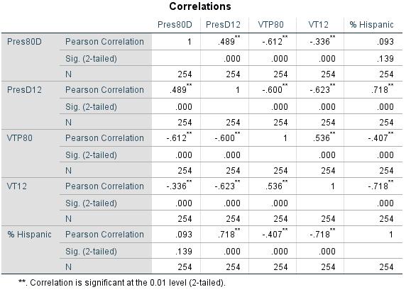
Figure 12: Matrix Correlation

Conclusion

We have seen a general pattern in this analysis; counties with high percentages of Hispanics do not vote in high numbers but when they do vote it is primarily for the democrat candidate. Voter turnout is higher in areas where there are lower percentages of people voting for democrat candidates. These patterns follow the proportions of Hispanics and non Hispanics living in Texas. Hispanics tend to be concentrated in the western counties and along the border of Mexico while non-Hispanics tend to concentrated in the panhandle, central and eastern counties in Texas. Voter turnout is low statewide but is especially low among Hispanics. To determine what causes this low turnout among Hispanics would require additional analyses as correlations and spatial autocorrelations cannot be used to infer causes of the linear relationships observed in this report. They do tell us, however, that there are relationships between these variables that are quite interesting that can guide additional research.  

Assignment 4-Hypothesis Testing
Goals of Assignment 4
Distinguish Between a Z- and T-Test
Calculate a z and t test
Use the Steps of Hypothesis Testing
Make Decisions About the Null and Alternative Hypotheses
Utilize Real-world Data Connecting Stats and Geography

Introduction

T-Tests: T-tests are used to test the mean of a sample population against a mean of a hypothesized population to determine if there is a difference. T-tests are used when you do not know the hypothesized population's standard deviation and when the sample population's size less than 30. 
The t-test tests whether the samples form a normal distribution or not and is based on Degrees of Freedom (the number of observations n-1, which is the degree to which a calculated statistic can vary).

Z-Test: Z-tests are similar but are used when the sample population's size is greater than 30 and the hypothesized population's standard deviation is known. The z-test is based on a sample that has a normal distribution.     

Hypothesis Testing Steps

State the Null: The null hypothesis is that of no difference, that there is no difference between the sample and hypothesized means.

State the Alternative Hypothesis: The alternative hypothesis is that of difference, that there is a difference between the sample and hypothesized means.

Choose a Statistical Test: In this assignment, we choose between the t- and z-tests, which are dependent upon sample sizes.

Set the Significance: The significance level is the probability of a Type I Error occurring. A Type 1 error is when we reject the null when we should not (a false positive). Significance can be set at any level you choose, but the usual levels of significance are 95% and 99%. This means that there is either a 95% or 99% chance that a Type I error will not occur.It also means that the calculated statistic would result in a false positive 5 or 1 times out of 100. These tests are either one-tailed or two-tailed. We use a two-tailed test when direction is not known and a one-tailed when direction or standard is given. When using a two-tailed the probability of a Type I Error occurring (5 times for a 95% significance level) will be divided in half. So, a 95% significance level would be set at 2.5% at both the left and ride sides of the distribution curve. A degrees of freedom and z-score chart are used to determine critical values.

Calculate Test Statistic: The equations used for this assignment are presented in Figures 3 and 4. A sample calculation of a t-value is in the ground nuts example, step 5. As you can see the formulas are identical.

Make a Decision Regarding the Null Hypothesis: Our degrees of freedom and significance levels determine our Critical Intervals and Critical Values. Critical Intervals are the range of numbers that fall between significance levels. For example, if our calculated statistic falls in this range we fail to reject the null as there is no difference. The opposite is true; if the calculated statistic falls outside of this range we would reject the null as there is a difference. The Critical Value is the "cutoff" value in that these are the numbers on each end of the critical intervals. Figure 1 portrays these ideas; the z-stat of 2.2 falls outside of our critical value so we would reject the null in this case.    

Figure 1: Critical Values and Intervals

(Ryan Weichelt)

Part I: T and Z Tests

1.

Figure 2: Z and T Test Exercise Results

2. A Department of Agriculture and Live Stock Development organization in Kenya estimates that yields in a certain district should approach the following amounts in metric tons (averages based on data from the whole country) per hectare: groundnuts. 0.55; cassava, 3.8; and beans, 0.28.  A survey of 23 farmers had the following results:

Figure 3: Data Table of Farmer Showing Sample Mean, µ, and Hypothesized Mean, µh.

Ground Nuts

1. State the Null: There is no difference between the farmer sample mean and national mean in ground nut production.

2. State the Alternative Hypothesis: There is a difference between the farmer sample mean and national mean in ground nut production.

3. Choose Statistical Test: As n<30, a two-tailed t-test will be used. Will be used for entire problem and will not be listed separately for the cassava or beans problems. 

4. Set Significance Level: Significance level is set to 95% for these analyses. With degrees of freedom equal to 22 and a two-tailed test,  the critical values will be -2.074 and 2.074 will be used for entire problem and will not be listed separately for the cassava or beans problems.

5. Calculate Test Statistic: 

Figure 4: T-Test Equation

(Ryan Weichelt)

Using the formula (Figure 4) and the data found on Figure 3 and an n of 23, the calculation resulted in a t-statistic of -.6667, after performing the following operations: .51-.55, divided by .3/square root of 23. This is used for the initial problem only as an example.

6. Make Decision Regarding the Null Hypothesis: In this case, we fail to reject the null as our calculated t-statistic did not exceed the critical values of -2.074 and 2.074. There is no difference between the sample mean (farmer survey sample mean) and the hypothesized mean (national production mean).

Probability Value of Calculated Answer: The probability of this calculated value is 0.75400, or 75.4%. The probability is 2.5%, so the null hypothesis was not rejected as 24.6% is greater than 2.5%.

Cassava 

1. State the Null Hypothesis: There is no difference between the farmer sample mean and the national mean in cassava production. 

2. State the Alternative Hypothesis: There is a difference between the farmer sample mean and the national mean in cassava production.

3. Calculate Test Statistic: This calculation resulted in a t-statistic of -2.667, using data found on Figure 1 and the formula in Figure 2, with an n of 23. 

4. Make Decision Regarding the Null Hypothesis: In this case we reject the null as our calculated 

t-statistic exceeded the critical values of -2.074 and 2.074. There is a difference between the sample mean (farmer survey sample mean) and hypothesized mean (national production mean).

Probability Value of Calculated Answer: The probability of this calculated value is .99311, or 99.311%. The probability is 2.5%, so the null hypothesis was rejected as .689% is less than 2.5%.

Beans

1. State the Null Hypothesis: There is no difference between the farmer sample mean and the national mean in bean production.

2. State the Alternative Hypothesis: There is a difference between the farmer sample mean and the national mean in bean production.

3. Calculate Test Statistic: This calculation resulted in a t-statistic of 1.6667 using the data found on Figure 1 and the formula in Figure 2, with an n of 23.

4. Make Decision Regarding the Null Hypothesis: In this case, we fail to reject the null hypothesis as our calculated t statistic did not exceed the critical values of -2.074 and 2.074. There is no difference between the sample mean (farmer survey sample mean) and hypothesized mean (national production mean).

Probability Value of Calculated Answer: The probability of this calculated value is .94768, or 94.768%. The probability is 2.5%, so the null hypothesis was not rejected as 5.23% is greater than 2.5%.

Results

According to the t-tests performed, the sample farm's production of beans and ground nuts was not statistically different than the national production mean for these products. There was, however, a statistically significant difference in cassava production; the sample's mean was lower than the national mean. The t-tests tells us that there is a difference here but does explain what that difference is. The sample means for ground nuts and cassava were both below the national production mean but only cassava was statistically significant. The sample mean was higher than the national mean for beans production but was not found to be statistically significant.

3. A researcher suspects that the level of a particular stream’s pollutant is higher than the allowable limit of 4.4 mg/l.  A sample of n= 17 reveals a mean pollutant level of 6.8 mg/l, with a standard deviation of 4.2.  What are your conclusions?  (one tailed test, 95% Significance Level) Please follow the hypothesis testing steps.  What is the corresponding probability value of your calculated answer.

1. Null Hypothesis: There is no difference between the sampled stream's mean pollutant level and the allowable limit.

2. Alternative Hypothesis: There is a difference between the sampled stream's mean pollutant level and the allowable limit.

3. Choose Statistical Test: As n<30 a t test will be used (Figure 1). 

4. Set Significance Level: Significance is set at 95%, one-tailed test as there is a set standard for pollutant levels. The critical value for this test with 16 degrees of freedom is 1.746.

5. Calculate the Statistic: This calculation resulted in a t statistic of  2.355.

6. Make Decision Regarding the Null Hypothesis: Based on our calculated t statistic of 2.355 we will reject the null as this observed value exceeds the critical value of 1.746. There is a difference between the sample mean (stream samples) and the hypothesized mean (allowable limit of pollutants in streams).

Probability Value of Calculated Answer: The probability of this calculated value is 0.98660, or 98.66%. The probability is 5%, so the null hypothesis was rejected as 1.34% is less than 5%. 

Part II: Utilizing Real-World Data Connecting Statistics and Geography

1. State The Null Hypothesis: There is no difference between the sample mean, home values in the City of Eau Claire, and the hypothesized mean, home values in Eau Claire County outside of the city of Eau Claire.

2. State the Alternative Hypothesis: There is a difference between the sample mean, home values in the City of Eau Claire, and the hypothesized mean, home values in  Eau Claire County outside of the city of Eau Claire.

3. Choose Statistical Test: As n>30, a z-test will be used to calculate this statistic. The critical values for this test is -1.96 and 1.96..

4. Choose Significance Level: The significance level is set at 95%; a two-tailed test is used as the direction is unknown.

5. Calculate Test Statistic: 

Figure 5: Z-test Equation

(Ryan Weichelt)

The overall mean home values in Eau Claire County by block group is $169,438 (hypothesized mean) and the mean home values in the city of Eau Claire by block group is $151,876 (sample mean).The standard deviation for our sample is 49,706.9 and the number of observations in our sample is 53. This resulted in a z-statistic of -2.57 using the equation in Figure 5. 

6. Make a Decision Regarding the Null Hypothesis: As our calculated z-statistic falls below our critical valule of -1.96, we reject the null hypothesis.

Probability Value of Calculated Answer: The probability of this calculated value is .9949, or 99.49%. The probability is 2.5%, so the null hypothesis was rejected as .51% is less than 2.5% 

Results 

It was found that home values in the city of Eau Claire are significantly lower than Eau Claire County as a whole. As can be seen in Figure 5, the lowest values are all located within the city limits of Eau Claire (upper northwest corner with black border). The homes with the lowest values are located near the center and north of the center of the city, with more valuable homes being located on the outer edges of the city limits. No average home values outside of the city of Eau Claire are below $122,260. Figure 6 shows the same information but is presented using the Standard Deviation classification method. Most of the block groups with a negative standard deviation are located within the City of Eau Claire's limits, with values approaching -1.5 standard deviations from the mean in 3 areas. This means that they are further from the mean on the negative standard deviation side and have lower average values. The calculated z-statistic tells us that there is a difference but does not explain what that difference is. Several interesting questions could be asked. Are lot sizes larger outside of the city, on average? Is there a difference in size between homes in Eau Claire and the rest of the county, on average? Do "bad neighborhoods" have an influence on values? How many homes are in each block group? These questions are simple but, given more data, are easily answerable. There are several other questions that could be asked but would require more than a z-score to answer, such as "Do the location city dumps, waste treatment plants, or industrial areas affect average home values as a function of distance?"

Figure 5: Average Home Values in Eau Claire County

Figure 6: Average Home Values in Eau Claire County, Standard Deviation Classification Method

Assignment 3

Goals of Assignment 3

Add a Field in ArcMap

Calculate Z-Scores From Data in ArcMap

Use Probability to Predict Occurrences of a Given Percentage

Create a Report Connecting all of the Data

Introduction

Foreclosures are "the action of taking possession of a mortgaged property when the mortgagor fails to keep up their mortgage payments" (Google Dictionary), and this spatial analysis is being conducted as a response to an increasing concern among Dane County officials due to increasing foreclosure numbers in the county. A census tract are "small, relativity permanent statistical subdivisions of a county, uniquely numbered with a numeric code" (United States Census Bureau) and average about 4,000 people per tract. The purpose of this project is to determine the z-scores of three census tracts, to determine the number of foreclosures that have an 80% and 10% likelihood of occurring, to determine whether the number of foreclosures will increase in 2013, and to perform a spatial analysis to determine changing patterns in foreclosures by census tract in Dane County, Wisconsin, from 2011-2012.

Methodology

To determine z-scores, the probability of an increase in foreclosures in 2013, and the spatial relationship of foreclosures in Dane County between the years 2011 and 2012, three operations were performed: a hand calculation of z-scores, a hand calculation of the probability of an increase in foreclosures in 2013, and a spatial analysis of foreclosure data mapped using ArcMap. A z-score is simply the distance, in standard deviations, above or below the mean that a raw score falls on, as seen in Figure 1 (two example z-scores circled in red and blue) which allows us to explain the probability of an observation occurring. Z-scores of census tracts 25, 108, and 120.01 were calculated using data for 2011 and 2012, while the probability of an increase in foreclosures used 2012 foreclosure data exclusively. The formula used to calculate z-scores and probability is shown in Figure 2, where z is the z-score, X is observation, μ is the mean, and σ is the standard deviation for this data set. The observation, mean, and standard deviations data were found using ArcMap classification statistics. The final task was mapping the changes in foreclosures for the entirety of Dane County. A new field was added in ArcMap, named change, representing the difference (positive or negative) in the number of foreclosures observed between 2011 and 2012. Another chloropleth map was then created using the Count2012 data that comprises the total number of foreclosures in Dane County in 2012 (Figure 6). Two additional maps (Figures 7 and 8), using the Count2011 and Count2012 data columns in ArcMap, were then created in ArcMap and displayed the total number of foreclosures using the standard deviation classification method. This allowed for a connection between z-score calculation in census tracts 25, 108, and 120.01 and the data displayed on these maps. The 2011 foreclosure map portrayed the data in four standard deviation classes while the 2012 foreclosure map portrayed the data in five standard deviation classes. All analyses utilized information provided by Dr. Ryan Weichelt and consisted of geocoded addresses of disclosures and all census tracts that contain these addresses in Dane County and a z-score chart (Figure 3). 

Figure 1: Normal Distribution with Z-Score Distribution    

(http://www.statisticshowto.com/when-to-use-a-t-score-vs-z-score/)

Figure 2: Z-Score Formula
(https://openlab.citytech.cuny.edu/2013-spring-mat-1272-reitz/2013/05/page/2/) 

Figure 3: Z-Score Chart

Results

The z-scores for census tracts 25, 108, and 120.1 were calculated (using Figures 2 and 3) and the results are portrayed in Figure 4. In 2011 the mean number of foreclosures in Dane County census tracts was 11.39 while the standard deviation was 8.78. Census tracts 108 and 120.01 both have more foreclosures than the mean whereas census tract 25 falls below the mean (Figure 7). These z-score values change when looking at the 2012 data (Figures 4 and 8). The mean increased to 12.3 (due to an overall increase in the number of foreclosures in 2012 over 2011) and the standard deviation  increased to 9.9, reflecting a slight spreading of data about the mean. Census tract 25 moves farther from the mean, reflecting a decrease in foreclosures, census tract 108 moves closer to the mean, also representing a decrease in foreclosures, while 120.01 increases drastically so that it is now 3 standard deviations from the mean (Figure 8). The number of foreclosures that is likely 80% of the time is 3.98 while the number that is likely 10% of the time is 24.97 (Figure 4). Figure 5 represents the total changes in the number of foreclosures in census tracts between 2011-2012 using the Jenks Natural Breaks classification method. There was an overall increase in foreclosures in Dane County from 2011-2012 ((evidenced by the increase in mean mentioned previously), but this increase is not distributed evenly among the census tracts and a spatial pattern emerges. The highest numbers of observed increases (11-16), occurred in seven census tracts (including census tract 120.01) on or near the outer edges of Dane County, primarily in the east. More moderate increases (1-9) occurred in or near the center of the county and on the western edge of Dane County. Decreases in foreclosure rates were most pronounced (-14--6) in census tracts 120.02 and 132 (among others) and all decreases generally run along a line running northeast to southwest from census tract 117 to census tract 126. Using Figure 5, we observe that census tracts 25 and 108 had 2-5 less foreclosures in 2012 while census tract 12.01 had 11-16 more foreclosures. Figures 7 and 8 portray the total number of foreclosures using the standard deviation classification method by year. These maps, used in conjunction, show that the center of Dane County is generally below the average number of foreclosures per census tract, a higher than average south of the center of the county, and that the eastern and northern boundaries have a higher than average number of foreclosures. Figure 6 represents the spatial distribution of the total number of foreclosures in Dane County in 2012. Figure 6 has a spatial pattern that matches Figure 5 in several ways, including a generally low number of foreclosures in census tracts running from the northeast to the southwest, with a very low number of foreclosures located in the center of Dane County, and higher numbers observed along the eastern and northern edges of Dane County. Figure 6 can be used in conjunction with Figure 5 in determining where we observe the greatest increases in the number of foreclosures between 2011-2012 (Figure 5) and where the number of foreclosures is the greatest in 2012 (Figure 6). Census tracts 116, 120.01, and 119 are among those that fit these criteria. Census tracts 114.01 and 114.02, while having high numbers of foreclosures in 2012, have not experienced as high of an increase compared to the tracts mentioned in the preceding sentence, and, therefore, do not fit with the criteria that has been set by the author (which can be adjusted; see conclusion).  

Conclusion

The results show that not all census tracts are experiencing high numbers of foreclosures or an increase in foreclosures. There is a pattern of higher than average foreclosures on the northern and eastern boundaries of the county and south of Dane County's center. Lower than average foreclosures are generally found in the center of the county and to the immediate east of the county center. These findings are significant as that they can be used to guide county officials to where help may be most needed. Recommendations will be made to county officials that several census tracts, including tracts 116, 120.01, and 119, should be of immediate concern as they have had large increases between 2011-2012 along with high total foreclosures in 2012. A focus has been limited to counties that have a high number of foreclosures in 2012 and high increases from 2011-202 as county resources may not be able to effectively help and support numerous families with things such as financial aid, temporary housing, or nutritional needs. If there are enough county resources, an exception could be made. Some census tracts, such as tract 129 (Figure 6), have gone from low single to double digits in one year (2 to 16 in census tract 129's case), or have a high overall number of foreclosures, such as that observed in census tracts 114.01 and 114.02 (Figure 6). The reason for the increase in foreclosures is not known as limited data was utilized answering the study questions but it would be fair to assume that an increase in the number of foreclosures would be observed in 2013 for the following reasons: we observe an increase in total foreclosures from 2011-2012, which could suggest a trend, an economic downturn could occur resulting in even more foreclosures, the standard deviation map of 2012 (Figure 8) has an additional class that is >2.5 standard deviations from the mean, containing 3 census tracts, which is unlikely if the number of foreclosures observed is simply due to chance (3/106 or 2.8% against 1.6% expected, Figure 1). We also have a positively skewed distribution (as evidenced by the lower than expected standard deviation values on the left,<-0.5, of the curve as compared to higher than expected values on the right, >2.5) as seen in figure 8), there fewer census tracts that fall below <-0.5 standard deviations from the mean in 2012 as compared to 2011 (Figures 7 and 8), and there is always the possibility that we may see an increase due to chance as a normal distribution is a probability distribution. There, however, is no way to confirm that there will be an increase without additional data.        

Z-Score Results

	2011	2012
Census Tract 25	-0.61	-.94
Census Tract 108	2	1.48
Census Tract 120.01	1.78	3

Figure 4: Z-Score Results for Selected Tracts, 2011 and 2012 Data

Probability Results

The number of foreclosures exceeded 80% of the time is 3.98 foreclosures, meaning that this number is very likely to be observed in a census tract.

The number of foreclosures exceeded 10% of the time is 24.97 foreclosures, meaning that this number is very unlikely to be observed in a census tract.

   

Figure 5: Changes in Foreclosures Between 2011-2012 in Absolute Values

Figure 8: Foreclosure Totals, 2012 Data

Figure 7: Foreclosures by Census Tract, 2011, Standard Deviation Classification Method

Figure 8: Foreclosures by Census Tract, 2012, Standard Deviation Classification Method

Assignment 2
Goals of Assignment 2
Increase Familiarity with Definitions of Descriptive Statistics
Increase Familiarity with Statistical Methods
Increase Familiarity with Computer Programs

Part 1
Methods: Range, mean, median, mode, kurtosis, skewness, and standard deviation were defined by the author, in his own words. Data supplied by Dr. Ryan Weichelt was used to hand calculate a standard deviation for two sets of data: the first standard deviation was calculated using a sample of student's standardized test scores from Eau Claire North High School and the other standard deviation was calculated using a sample of student's standardized test scores from Eau Claire Memorial. Microsoft Excel was then used to calculate the range, mean, median, mode, kurtosis, skewness, and standard deviation for the Eau Claire North and Eau Claire Memorial data samples. These results were then used to answer the following question; "Should Eau Claire North teachers worry about not having the highest test grade?"

Definitions

Range: The range is the difference between the highest and lowest scores; max score - low score.

Mean: The mean is the calculated average of all observations, found by adding all observations together then dividing by the total number of observations.

Median: The median is the midpoint of the data set; half of the observations fall above and half fall below this point. If the total number of observations is odd, it is simply the middle number in the data set and, if the total number of observations are even, it is the average of the two middle observations.

Mode: The mode is the most frequently occurring data point found in a set of observations.

Kurtosis: Kurtosis (Fig. 1) is the shape of the distribution curve and can be mesokurtic (normal), leptokurtic (peaked), or platykurtic (flat). A value greater than 1 is considered leptokurtic while a value less than -1 is considered platykurtic. Curves that are lepto- or platykurtic have this shape as 68% of the observations one standard deviation above and below the mean have to fit in that area (Fig. 2). Leptokurtic distributions have smaller standard deviations as there are more observations near the mean while platykurtic distributions have larger standard deviation values.

Figure 1: Kurtosis

(http://grants.hhp.coe.uh.edu/doconnor/PEP6305/KurtosisPict.jpg)

Figure 2: Normal Distribution

(http://img.tfd.com/dorland/distribution_normal.jpg)

Skewness: Skewness (Fig. 3) is the measure of the asymmetry of a distribution curve due to a higher-or lower-than-expected number of observations that fall into the positive or negative ends of the curve; if  positive there is an extended tail to the positive side (due to more observations that are lower-than-expected) and, if negative (due to more observations that are higher-than-expected), an extended tail to the negative side. A value below 1 and above -1 is considered normal.

Figure 3:Skewness

(https://www.isobudgets.com/wp-content/uploads/2015/10/skewness.jpg)

Standard Deviation: The standard deviation (Fig. 4) is the distribution/distance of scores about/from the mean, found by subtracting the mean from each observation, squaring the result, then finding the square root of the sum of these results after dividing by N or n-1. In this assignment n-1 was used as this is a sample population standard deviation.

Figure 4: Sample and Population Standard Deviation Equations

(http://dsearls.org/courses/M120Concepts/ClassNotes/Statistics/StandardDeviation2a.gif)

Hand Calculation

Eau Claire North Test Score Data Hand Calculation

Figure 5: Eau Claire North Data

Eau Claire Memorial Test Score Data Hand Calculation

Figure 6: Eau Claire Memorial Data

Results

Eau Claire North Test Scores

Eau Claire Memorial Test Scores

This data suggests that teachers at Eau Claire North have no reason to worry about being fired because their students have lower test scores than students at Eau Claire Memorial. The four  descriptive statistics that are best for determining this are the range, median, mean and kurtosis. I chose these for the simple fact that they portray score differences in a manner that is easy to explain to people with little knowledge of descriptive statistics. EC North students have a lower range (83 compared to 91) which shows us that their test scores are less widely dispersed than the EC memorial students scores were; i.e. the lowest score attained by a student at North (111) was closer to the highest score attained by another student at North (194) than the difference between the lowest (107) and  highest (198) scores attained at Memorial. This may suggest that the North students taking the test were better prepared at all levels of ability as compared to the students at Memorial. The median was higher at North (164.5) than at Memorial (159.5). This tells us that half of the students at North who took this exam in this sample had a score higher than 164.5 and half had a score lower than 164.5, compared to Memorial's median of 159.5. The mean test scores in this sample show that North, with a 160.92 average, had a higher mean test score than Memorial, at 158.54, did. Kurtosis refers to the shape of the distribution; the shape of the distribution curve based on the sample of test scores at North (-.56) is between -1 and 1 and is normal. The shape of the distribution curve based on the test score samples from Memorial is less than -1 (-1.17) and is considered platykurtic. This flatness of the curve is due a larger standard deviation value (27.16) and reflects the extreme disbursement of scores from the mean; we have less scores near the mean score of (158.54) than we observe based on the sample from North (160.92), i.e. the scores at north were closer to the mean. The students at North, on average, performed better on this standardized test. These statistics show that the teachers and students at North are doing quite well and public perceptions are not only unjustified but probably incorrect. This analysis was done using a sample of test scores from both schools using descriptive statistics; we are describing what we see and can make assumptions about this data but we cannot make any inferences regarding it. 

Part 2

Methods: The shapefile used in Assignment 1 was added to a blank map in ArcGIS and a Microsoft Excel spreadsheet, provided by Dr. Ryan Weichelt containing Wisconsin population data by county, was joined to the shapefile based on countyGeo_id. Three spatial statistic analyses were performed: a geographic mean center of Wisconsin (Toolbox/Spatial Statistics/Measuring Geographic Distributions/Mean Center), a weighted mean center of population using 2000 Wisconsin county population data (Toolbox/Spatial Statistics/Measuring Geographic Distributions/Mean Center/Weight/2000), and finally a weighted mean center of population using 2015 Wisconsin county population data (Toolbox/Spatial Statistics/Measuring Geographic Distributions/Mean Center/Weight/2105). 

Mean Center: The mean center is a spatial measurement of central tendency; in the map below it is represented by the red point which represents the geographical center of the state of Wisconsin found by averaging X and Y values (latitude and longitude).

Weighted Mean Center: Weighted mean centers are concerned with the frequencies in data sets; in the map below mean centers were weighted by population. More populous areas (counties) have a higher number of people and therefore have a heavier weight which pulls the geographic mean center toward the direction of more populous counties.

Results: The green point represents the weighted mean center of population in 2000, and the blue, of 2015. Both points are pulled to the southeast of the geographic center of Wisconsin, which is the red point, as the southern and eastern regions of Wisconsin have a higher population than the northern and western parts of the state. This is due to high populations in cities such as Milwaukee (southeast corner of the state), Madison (south-central), and Green Bay (east-central), for example. We observe, however, that the weighted mean center of population in 2015 has been pulled slightly to the southwest of the weighted mean center of population observed in 2000. An explanation for this is slight increase in county populations in the southern and western parts of the state that is greater than the increase in the northern and eastern counties in the state.